Random variables in statistics

The world is full of uncertainties, and mathematics provides us with tools to understand and predict them. A random variable plays a central role in this context—a concept from probability theory. But what exactly is a random variable, why is it important, and how can we use it?

Basic Understanding of a Random Variable

A random variable is a function that assigns numbers to the possible outcomes of a random experiment. This allows us to quantify random processes and analyze them mathematically.

Formal Definition

A random variable X is a function that assigns a real number to each element ω (lowercase omega) of a sample space Ω (uppercase omega):

An example helps clarify this abstract definition.

Example: Rolling a Die

Imagine you throw a die:

The sample space $\Omega$ contains all possible outcomes: {1, 2, 3, 4, 5, 6}.
A possible random variable could represent the number rolled, that is:

In this case, the value of the random variable $X$ directly corresponds to the outcome of the die roll.

Types of Random Variables

Random variables can broadly be divided into two categories: discrete and continuous random variables.

1. Discrete Random Variables

A random variable is called discrete if it can take only finitely many or countably infinitely many values.

Properties

The values are clearly distinct from one another.
The probability that a specific value is assumed can be described using a probability mass function:

Examples

Rolling a die: The numbers on the die (1 to 6) are discrete values.
Number of customers: A shop receives 0, 1, 2, … customers per day.

2. Continuous Random Variables

A random variable is called continuous if it can take any value within an interval.

Properties

There are infinitely many other possible values between any two values.
Probabilities are defined using a probability density function. The probability that the random variable takes exactly one specific value is theoretically zero. Instead, we consider probabilities for intervals.

Examples

Height: A person can be 170.5 cm or 170.503 cm tall.
Time until a device fails: The time span is continuous.

Why Are Random Variables Important?

Random variables are at the heart of many applications of statistics and probability. They provide a way to model and predict real-world phenomena mathematically. Here are some important reasons why they are so central:

Quantifying Uncertainty: Random variables make it possible to measure and analyze uncertainty.
Mathematical Modeling: They help describe complex processes mathematically, such as weather, stock prices, or genetic inheritance.
Basis for Probability Distributions: Every random variable has a distribution that shows how likely different outcomes are.
Decision-Making: Random variables are indispensable in areas such as actuarial mathematics, finance, and risk management.

Distribution of Random Variables

The distribution of a random variable describes how the probabilities are distributed across the possible values. There are different types of distributions, which vary depending on the type of random variable.

Discrete Distribution

For discrete random variables, the probability distribution is described by the probability mass function (PMF). This function indicates the probability P(X = x) that the random variable X takes the value x.

Example: Coin Toss

Sample space: {Heads, Tails}
Random variable:

The probabilities are:

Continuous Distribution

For continuous random variables, the distribution is described by the probability density function (PDF). The probability that the random variable takes a value within an interval is calculated using the integral of the density function:

Example: Height

Sample space: All values within an interval, e.g., [150,200]
Probability density: A normal distribution could describe the probabilities for different heights.

Mathematical Properties of Random Variables

1. Expected value

The expected value (or mean) of a random variable indicates the value we can expect on average if we repeat the experiment infinitely many times.

2. Variance

The variance measures how much the values of a random variable vary around the expected value:

3. Standard deviation

The standard deviation is the square root of the variance and indicates the average deviation from the mean.

Visualizing random variables

Charts and graphs help us understand the behavior of random variables. Here are some common visualizations:

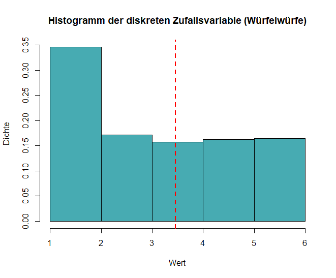
Histograms: Show the probability distribution of discrete random variables (see the example code in R below):

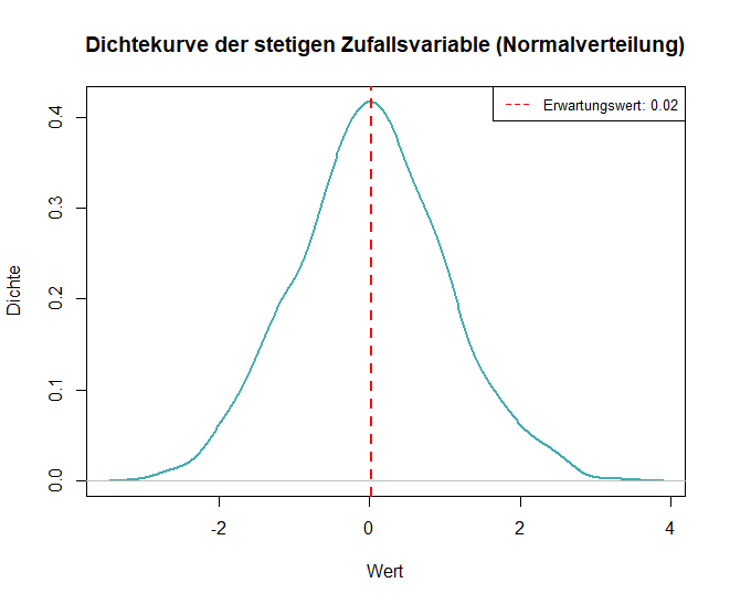
Density curves: Illustrate the probability density of continuous random variables (see the example code in R below):

Summary example in R

# Discrete random variable (e.g., dice rolls)
set.seed(123)
dice_rolls <- sample(1:6, size = 1000, replace = TRUE)

# Expected value, Variance and Standard deviation for the random variable
mean_discrete <- mean(dice_rolls)
var_discrete <- var(dice_rolls)
sd_discrete <- sd(dice_rolls)

# Continuous random variable (e.g., normal distribution)
set.seed(123)
continuous_data <- rnorm(1000, mean = 0, sd = 1)

# Expected value, Variance und Standard deviation for continuous random variable
mean_continuous <- mean(continuous_data)
var_continuous <- var(continuous_data)
sd_continuous <- sd(continuous_data)

# Histogram for discrete random variable
hist(dice_rolls, breaks = 6, probability = TRUE, col = "#47abb2",
     main = "Histogram of discrete random variable (dice rolls)",
     xlab = "Value", ylab = "Density")
abline(v = mean_discrete, col = "red", lwd = 2, lty = 2)
legend("topright", legend = paste("Expected value:", round(mean_discrete, 2)), col = "red", lty = 2, cex = 0.8)

# Density curve for the continuous random variable
plot(density(continuous_data), col = "#47abb2", lwd = 2,
     main = "Density curve for the continuous random variable (Normal distribution)",
     xlab = "Values", ylab = "Density")
abline(v = mean_continuous, col = "red", lwd = 2, lty = 2)
legend("topright", legend = paste("Expected value:", round(mean_continuous, 2)), col = "red", lty = 2, cex = 0.8)