
How old are the respondents? How satisfied are they with democracy? And do the means differ between women and men?
In this exercise, you will learn how to calculate key descriptive statistics for real survey data—with SPSS and R.
Aim of the exercise
- Calculation and interpretation of measures of central tendency (mean, median, mode)
- Analysis of measures of dispersion (standard deviation, range, IQR)
- Application in SPSS and R
- Understanding different types of variables
- Conducting comparisons between groups by gender
The data: ALLBUS 2021
We use the ALLBUS 2021 dataset (ZA5280) from GESIS. It contains nationally representative survey data from Germany.
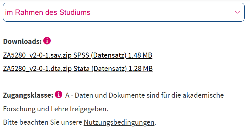
Download the SPSS file (.sav) (you need to register with GESIS beforehand, but registration is free and useful anyway). You can open it directly in SPSS or import it into R using the haven package:
library(haven)
dat <- read_sav("allbus2021.sav")
The variables
We will analyze five variables:
| Variable | Label in the dataset | Type |
|---|---|---|
| Age | age | Metric |
| Satisfaction | satdem* | Ordinal (Likert scale) |
| Educational attainment | educ | Ordinal/Categorical |
| Household income | inc* | Metric, skewed |
| Gender | sex | Categorical (groups) |
* Attention: Some “errors” have crept in here! Try to figure out which other variables you could take from the dataset! (Tip: The corresponding codebook on the GESIS website is very helpful for this!)
Your task
Calculate the measures of central tendency and dispersion that you know for the specified variables. Explore the data carefully to understand what numbers are actually being produced and how they should be interpreted (注意, there are several pitfalls here!)
Below you will find possible solutions and, in particular, a commented video that guides you through the process.
Step by step through the task
Solution video for R
Step 1: Calculate measures of central tendency
In R:
mean(dat$age, na.rm = TRUE)
median(dat$age, na.rm = TRUE)

#Alternatively, more compactly using the psych package
library(psych)
psych::describe(dat$age, na.rm = TRUE)
You can learn more about the psych package here .
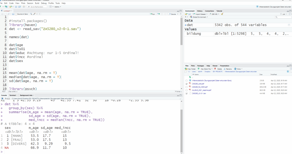
In SPSS:
- Menu: Analyze > Descriptive Statistics > Descriptives
- Select variable(s)
- Options: check Mean, Median, Mode
Step 2: Calculate measures of dispersion
In R:
sd(dat$age, na.rm = TRUE)
range(dat$age, na.rm = TRUE)
IQR(dat$satdem, na.rm = TRUE)
In SPSS:
- Menu: Analyze > Descriptive Statistics > Explore
- Under “Statistics,” you can select range, IQR, standard deviation.
Step 3: Grouped analysis by gender
In R:
library(dplyr)
dat %>% group_by(sex) %>%
  summarise(m_age = mean(age, na.rm = TRUE),
            sd_age = sd(age, na.rm = TRUE),
            med_inc = median(inc, na.rm = TRUE))
In SPSS:
- Menu: Data > Split File… > By gender (
sex) - Then, as above: calculate descriptive statistics
Step 4: Interpret the results
- Mean vs. median: Does a large difference indicate skewness?
- Dispersion: Is the group homogeneous or highly varied?
- Group comparisons: Are there systematic differences by gender?
- Which measures make the most sense for which variable?
Conclusion
This exercise will give you a feel for different statistics in real-world data—and how to analyze them quickly in SPSS and R.
If you like, expand the analysis by adding visualizations (boxplots, histograms) or try a different grouping variable (e.g., region or education).